World Models (Ha & Schmidhuber, 2018): A Complete Summary

1. The Core Problem the Paper Addresses

Reinforcement learning agents traditionally learn a policy directly from pixels, which has two major problems:

Poor sample efficiency — it requires an enormous number of interactions with the real environment.
End-to-end training is hard to decompose and hard to reuse.

This paper proposes: first let the agent learn to “understand how the world works,” then have it make decisions based on that internal understanding — and it goes on to verify a bold corollary: if this internal understanding is accurate enough, the agent can train entirely inside its own “imagination,” with no need for the real environment to be involved at all.

2. The Three Modules: V / M / C

The agent is split into three separately trained modules with a clear division of labor:

The V/M/C three-module architecture

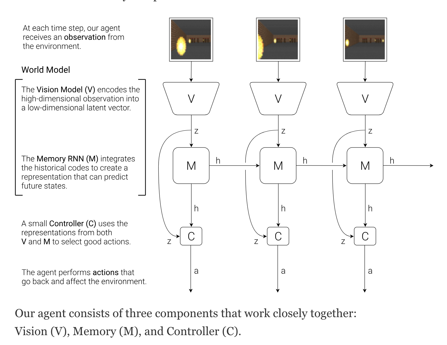
V (Vision): uses a VAE to compress each high-dimensional frame of image into a low-dimensional latent variable $z$ (32-dimensional in the paper, $D=32$ ).
M (Memory): uses an RNN + MDN to learn the environment’s transition dynamics, predicting what the next $z$ might look like.
C (Controller): an extremely simple linear model that maps $[z_t, h_t]$ directly to an action $a_t$ .

The feedback loop for action $a$ : in the diagram, the output $a_t$ from C is only drawn with a downward arrow (flowing to “the environment”), but this same $a_t$ also feeds back into M at the next step. The complete causal chain is:

C(t): (z_t, h_t) \rightarrow a_t \;\longrightarrow\; M: (z_t, a_t, h_t) \rightarrow h_{t+1} \;\longrightarrow\; C(t+1): (z_{t+1}, h_{t+1}) \rightarrow a_{t+1}

$a_t$ is C’s output at time $t$ , and at time $t+1$ it becomes an input M needs — the same variable, appearing at two different positions along the causal chain. This is the standard “agent-environment interaction loop.”

3. The V Module: How the VAE Works and Is Trained

3.1 VAE Structure: Encoder + Decoder, Trained Jointly

x \;\xrightarrow{\text{Encoder}}\; \mu(x),\sigma(x) \;\xrightarrow{\text{sample}}\; z \;\xrightarrow{\text{Decoder}}\; \hat{x}

The Encoder cannot be trained on its own — the reconstruction loss can only be computed with the Decoder’s help, and the training signal (gradient) originates on the Decoder side and is backpropagated all the way to the Encoder. Without the Decoder participating, the Encoder receives no feedback at all about “what encoding would actually be meaningful,” and the only remaining driving force (the KL term) would push it to degenerate into outputting $\mu=0, \sigma=1$ for every input.

3.2 The Loss Function: A Reconstruction Term Plus KL Regularization, Both Derived from the Same Mathematical Objective

\mathcal{L}_{\text{VAE}} = \underbrace{\|x-\hat{x}\|^2}_{\text{reconstruction loss}} + \underbrace{D_{KL}\big(q(z|x)\,\|\,p(z)\big)}_{\text{KL regularization}}

These two terms aren’t cobbled together arbitrarily — they’re derived from maximizing the evidence lower bound (ELBO) on $\log p(x)$ :

\log p(x) \geq \mathbb{E}_{q(z|x)}[\log p(x|z)] - D_{KL}\big(q(z|x)\,\|\,p(z)\big)

Reconstruction loss: forces $z$ to carry enough information about $x$ , or else the Decoder can’t reconstruct it.
KL regularization: forces the distribution $q(z|x)$ corresponding to each image to not stray too far from the prior $p(z)=\mathcal{N}(0,I)$ , preventing degeneration and keeping the latent space continuous, dense, and free of gaps.

There’s a natural tension between the two loss terms: the reconstruction loss wants to pull the encodings of different inputs apart, while the KL term wants to pull every encoding back toward the shared standard normal — the result of convergence is a compromise between the two.

3.3 What Exactly Is the Prior $p(z)=\mathcal{N}(0,I)$

$p(z)$ isn’t a vector — it’s a distribution defined over the entire $D$ -dimensional latent space, made up of $D$ mutually independent standard normal distributions combined together:

p(z) = \prod_{d=1}^{D}\mathcal{N}(z_d;0,1)

The figure below intuitively shows what 1,500 points sampled from this distribution look like when $D=2$ — the scatter cloud forms a rotationally symmetric circular pattern, and projecting each point onto a single coordinate axis and tallying the results gives you the familiar one-dimensional standard normal curve:

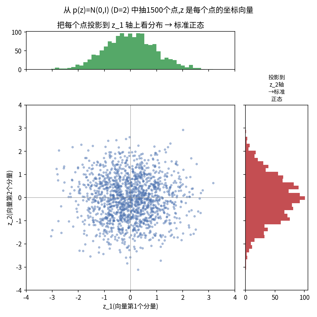
Scatter plot of a 2D standard normal distribution

This prior distribution itself carries no predefined semantics of any kind — it’s merely a mathematically convenient reference frame (the KL divergence has a closed-form solution, it supports the reparameterization trick, sampling is simple, and it’s isotropic with no preferred direction). What actually makes the latent space “meaningful” is the mapping the Encoder and Decoder jointly learn to coordinate during training.

3.4 “Which $z$ Does a Given Image Correspond To” — A Region, Not a Point

For each specific image $x$ , the Encoder outputs $\mu(x), \sigma(x)$ specific to that image, and the final $z$ is then sampled from $\mathcal{N}(\mu(x),\sigma(x)^2)$ — not the generic $\mathcal{N}(0,1)$ :

z = \mu(x) + \sigma(x)\cdot\epsilon, \qquad \epsilon\sim\mathcal{N}(0,1)

This sampling formula is the inverse operation of the standardization operation $z=(x-\mu)/\sigma$ : standardization “pulls” an arbitrary normal distribution back to standard normal, while this instead “transforms” a standard-normal sample $\epsilon$ into a distribution with a specified mean and variance — both exploit the fact that the normal distribution is closed under linear transformations. This technique is called the reparameterization trick: it converts the non-differentiable operation of “random sampling” into a linear operation that’s differentiable with respect to $\mu$ and $\sigma$ , letting gradients flow back through it smoothly.

Before vs. after training — when training starts, the Encoder’s weights are random and there’s no pattern to where images of the same category get encoded; once training converges, similar images get pushed into regions of the latent space that are close to one another, while the overall shape still stays close to the prior $\mathcal{N}(0,I)$ :

Before-and-after comparison of training

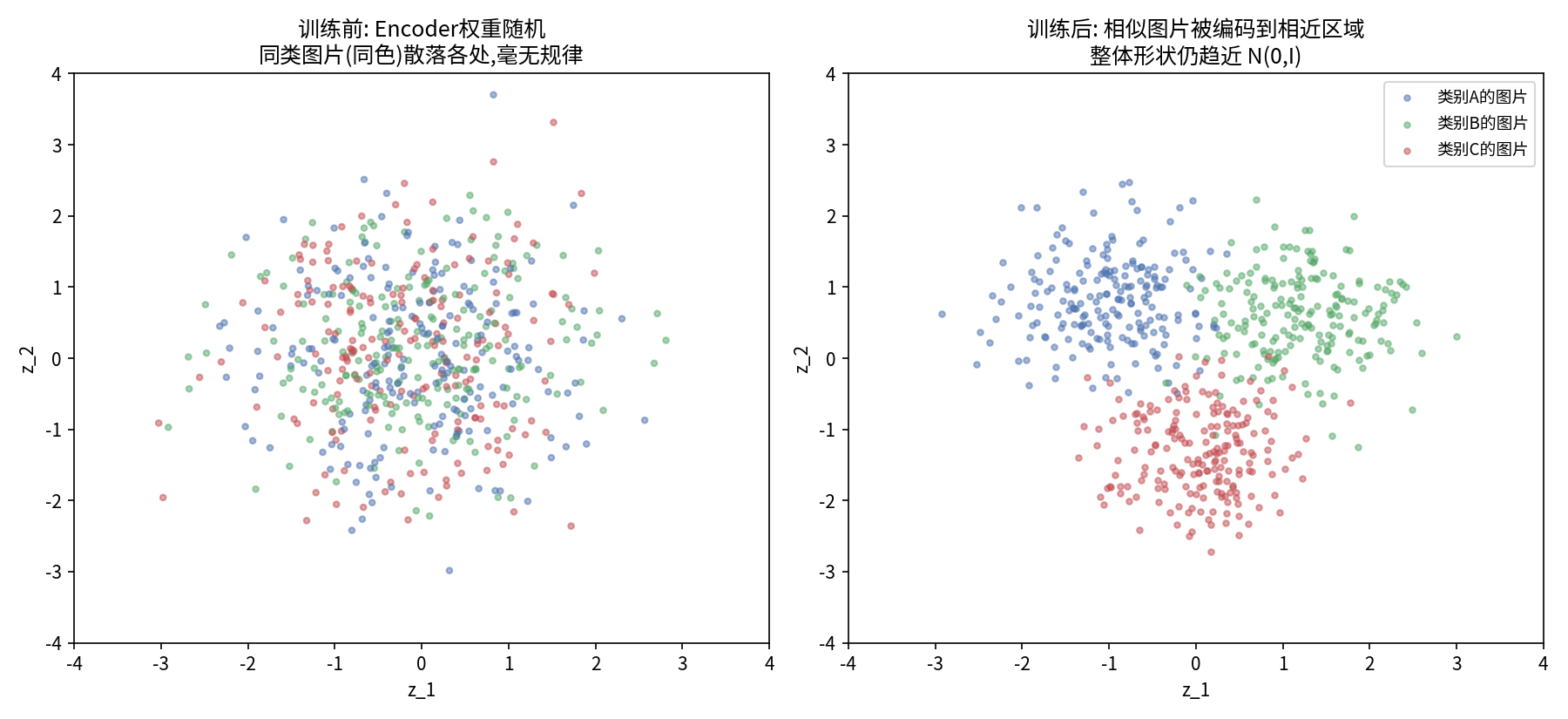
This “image → region” mapping isn’t designed or specified by hand — it’s the inevitable structure that gets “forced out” by the joint action of the reconstruction loss and the KL regularization. Exactly what semantic meaning each individual dimension represents typically can’t be determined in advance by a human — it usually requires post-hoc exploratory analysis (such as holding other dimensions fixed and sweeping one dimension while observing the decoded results) to interpret roughly what’s going on. Different training orders, weight initializations, and sampling noise will cause training to converge to different “orientations” of the latent space (for instance, the entire latent space can be arbitrarily rotated while the prior distribution remains unchanged), but as long as reconstruction quality is high and the latent space is continuous, these different versions of the VAE are functionally equally valid.

3.5 VAE vs. a Plain Autoencoder

	Autoencoder	VAE
Encoder output	A single deterministic vector	The parameters of a distribution $(\mu,\sigma)$
Training objective	Reconstruction loss only	Reconstruction loss + KL divergence
Latent space structure	Unconstrained, may have gaps	Continuous, dense, suitable for sampling
Can it be sampled to generate new content?	No (tends to produce garbage)	Yes

4. The M Module: RNN + MDN

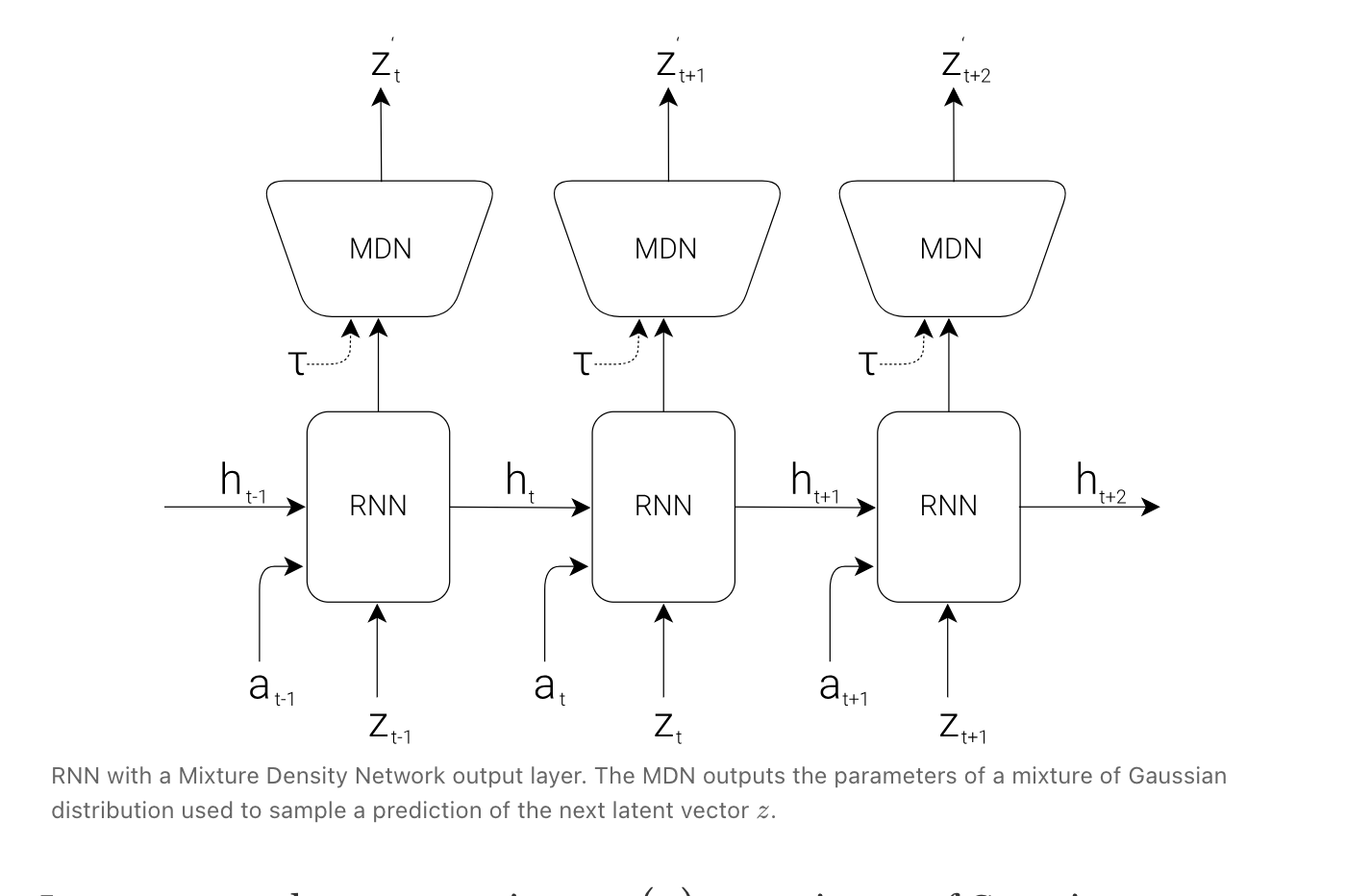
Detailed structure of the RNN and MDN

At each step, the RNN takes in $(z_t,a_t,h_{t-1})$ and updates the hidden state $h_t$ :

h_t = \text{RNN}(z_{t-1},a_{t-1},h_{t-1})

4.1 Why an MDN Instead of Direct Regression

The environment’s future is often multimodal (the same history may correspond to several plausible but drastically different continuations). If you regress directly to output a single $z$ , MSE training will lead the network to learn a “blurry average” that resembles nothing in particular. An MDN instead has the network output the parameters of a mixture-of-Gaussians distribution:

P(z_{t+1}\mid h_t) = \sum_{k=1}^{K}\pi_k\cdot\mathcal{N}(z_{t+1};\mu_k,\sigma_k^2)

Parameter	Count	Meaning	Constraint
$\pi$	$K$ values	Probability of selecting each component, shared across all dimensions	Softmax, non-negative and sums to 1
$\mu$	$K\times D$ values	The expected value of each dimension of $z$ , under each component	Unconstrained
$\sigma$	$K\times D$ values	The spread of each dimension of $z$ , under each component	Must be positive

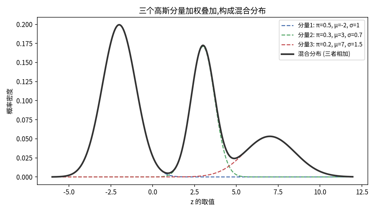
The figure below gives an intuitive picture of three Gaussian components combined by weight into a mixture distribution:

Three Gaussian components combined into a mixture distribution

4.2 Sampling: A Two-Step Process

k\sim\text{Categorical}(\pi_1,\ldots,\pi_K) \qquad\Longrightarrow\qquad z_d=\mu_{k,d}+\sigma_{k,d}\cdot\epsilon_d,\ \ \epsilon_d\sim\mathcal{N}(0,1)

First draw a single component according to $\pi$ (drawn just once for the entire $D$ -dimensional vector), then, within that selected component, sample each dimension independently — this is not a weighted average across components. $\pi$ is only responsible for the “selection” step; once a component is chosen, $\pi$ plays no further role in the computation. This is exactly what allows an MDN to express multimodality instead of degenerating into a blurry average.

4.3 Training: Teacher Forcing

During training, the RNN’s input at every step is always the real $z_{t-1}$ (encoded from a real observation by V), never a $z'$ sampled by the model itself. The loss function is the negative log-likelihood:

\mathcal{L}_M = -\log\left(\sum_{k=1}^K \pi_k\cdot\mathcal{N}(z_t^{\text{real}};\mu_k,\sigma_k^2)\right)

At this stage, any $z'$ sampled from the MDN is used only to compute one loss value and then discarded — it never participates in subsequent forward passes. Training stays anchored to real data throughout, so there’s no issue of autoregressive error accumulation.

4.4 Inference: Turning the MDN’s Output Distribution into a Concrete Vector

At inference time, you don’t directly “process” density values — instead you run the standard sampling procedure to arrive at one concrete, deterministic vector:

pi = softmax(pi_logits / tau)          # tau: temperature parameter, controls randomness
sigma = exp(log_sigma) * sqrt(tau)
k = multinomial(pi, num_samples=1)     # step 1: pick a component
epsilon = randn_like(mu[k])
z_next = mu[k] + sigma[k] * epsilon    # step 2: sample the concrete vector

The temperature parameter $\tau$ : as $\tau\to 0$ , it tends toward “always pick the component with the largest weight, with almost no added noise” (similar to greedy decoding in an LLM); the larger $\tau$ is, the stronger the randomness. If $\tau$ is set too low during the “dreaming” phase, the generated virtual environment ends up too orderly, and the Controller ends up “exploiting loopholes” rather than learning a robust policy.

Analogy with LLMs: the MDN and an LLM’s next-token prediction are fundamentally the same kind of problem — both are cases of “the network outputs the parameters of a distribution, and at inference time you sample from it probabilistically to get a concrete output, using temperature to control the amount of randomness.” The only difference is that an LLM faces a discrete choice over a finite vocabulary (Categorical + softmax), while the MDN faces a continuous real-valued space (a Gaussian mixture); both are trained directly against the real label using a loss (cross-entropy / negative log-likelihood), never relying on the model’s own sampled output.

5. The Complete Training Pipeline: Three Modules, Trained Separately, in Sequence

Stage	What’s trained	Data source	Role of $z$	Optimization method
1	V (VAE)	Real frames collected under a random policy	Encoding target	Reconstruction loss + KL (gradient descent)
2	M (RNN+MDN)	The real $z$ sequence encoded by V	Real $z$ used as input, teacher forcing	Negative log-likelihood (gradient descent)
3	C (linear controller)	Virtual trajectories generated by M (“dreaming”)	Autoregressively sampled $z'$ drives the whole trajectory	CMA-ES (an evolution strategy)

The core loop of the dreaming phase:

z_t' \sim \text{MDN}(h_t) \to h_{t+1}=\text{RNN}(h_t,z_t',a_t) \to z_{t+1}'\sim\text{MDN}(h_{t+1}) \to \cdots

C has an extremely small number of parameters (a few hundred, a linear model), and is trained with CMA-ES rather than a gradient-based reinforcement learning method: it maintains a distribution over parameters, and in each generation it samples candidate controllers, evaluates their cumulative reward, and updates the distribution’s mean and covariance based on performance, evolving generation by generation. Once trained, C is placed back into the real environment for testing, and it still performs well — proof that the agent can learn entirely detached from the real environment, relying only on internal imagination. Exactly how “cumulative reward” gets computed here, and whether training actually happens in the real environment or in a dream, is covered in detail in section 6.

6. Where Do Action and Reward Actually Come From

These are two easily overlooked but indispensable details that make the entire training pipeline actually work.

6.1 During V and M Training: Actions Are Generated by a Random Policy

While collecting data to train V and M, the paper uses a completely random policy to explore the environment — no intelligence is needed at all; at every step, an action is simply sampled at random from the action space:

CarRacing (continuous actions): steering, acceleration, and braking are three continuous values, randomly sampled each step.
VizDoom (discrete actions): one action is randomly chosen from a small finite set of options.

The goal at this stage is only to expose V and M to a sufficiently diverse set of frames and state transitions — there’s no need for the behavior to “look smart.” When the community reproduced this, they found that pure frame-independent white-noise actions would send the car off the track very quickly, exploring too narrow a range, so it’s common instead to use a temporally correlated (“Brownian-motion-style”) random policy, letting the action drift smoothly over time in order to collect more coherent, more representative trajectories.

6.2 During C Training: Where Reward Comes From Varies by Experiment

CarRacing: C is trained directly inside the real environment, and the reward is exactly the reward function built into the Gym environment (number of track tiles visited, time taken) — there’s no question here of “how to compute a reward inside a dream.”

VizDoom (the experiment that’s genuinely “trained entirely inside a dream”): this environment has no explicit reward of its own, so the paper redefines the reward as the number of time steps survived. For this definition to hold equally well inside a dream, the M module is extended to additionally predict a “done” (whether the agent has died) signal, output alongside the distribution predicting $z_{t+1}$ :

h_t=\text{RNN}(z_{t-1},a_{t-1},h_{t-1}) \;\longrightarrow\; \big(P(z_t\mid h_t),\ P(\text{done}_t\mid h_t)\big)

While dreaming, as soon as this signal indicates “death,” the virtual trajectory terminates — however many steps the trajectory ran for is exactly this evaluation’s cumulative reward, with no need to separately train a “reward-value prediction head” at all. This neatly sidesteps the problem of “how do you conjure up a reward value out of nowhere inside a dream.”

For environments with more complex reward structures (not just “alive or dead”), the more general approach — adopted by the later PlaNet and Dreamer work — is to add a reward prediction head to M as well, output alongside the $z$ prediction and the done prediction, trained with supervision from reward observed in the real environment; while dreaming, each step then directly outputs a predicted reward value, and these are summed to get the total reward.

Experiment	Where C is trained	Source of reward
CarRacing	Real environment	The environment’s built-in reward function, read directly
VizDoom (dreaming experiment)	Entirely inside the virtual environment generated by M	Reward = number of steps survived, determined indirectly by M’s additionally predicted “done” signal

7. Why This Paper Matters

It decouples “perceptual compression, dynamics prediction, and decision-making” into three separately trained modules, substantially lowering both the training difficulty and the parameter count; more importantly, it’s the first paper to concretely demonstrate that “training inside imagination” is actually feasible.

This line of thinking directly inspired DeepMind’s later PlaNet and Dreamer series (which took “dream training” much further, doing multi-step rollouts entirely within the latent space, to the point of skipping the step of decoding back to pixels entirely), and it’s also one of the important sources behind “world models” becoming a hot topic again in large-model/generative-modeling research in recent years (as seen in Sora, Genie, JEPA, and others).